Chromotopy

The K-Theory of Endomorphisms

For the purposes of this post, I am going to assume that you are all familiar with the basics of Algebraic $K$-theory. If you’re not, just treat it as a black box, a gadget which takes in one of :

• a (simplicial) ring (spectrum)
• an augmented (simplicial) bimodule over a ring
• an exact category
• a Waldhausen category
• a small, stable $\infty$-category

and spits out a spectrum $K(\mathcal{C})$, such that $K(\mathcal{C})$ does the job of  ”storing all Euler characteristics” or “additive invariants”.

An important example is when $\mathcal{C}$ is the category of finitely generated projective modules over a ring $R$, and then we call this $K(R)$. It is a generally-accepted fact that the $K$-theory of rings is generically a very difficult and often useful thing to compute (knowledge of the $K$-groups of $\mathbb{Z}$, for example, would be quite valuable to many). In an ideal world, we would be able to understand the functor

$$A \mapsto \tilde{K}(A) = hofib(K(A) \rightarrow K(R))$$

on the category of algebras augmented over a given ring $R$, but this ends up being fairly intractable. One might hope that it would be easier to look at what happens when restricted to free augmented algebras, that is looking at the functor on (flat) $R$-bimodules

$$M \mapsto \tilde{K}(T_R (M)),$$

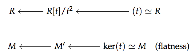
where $T_R (M)$ is the tensor algebra on $M$. This is pretty tough, but it turns out that we can do it. Let’s take a baby step first, and try to understand the K-theory of the “linearized” tensor algebra. The 1st Goodwillie derivative of the identity functor on augmented $R$-algebras is given by

$$P_1 (id) (A) = A / I^2 ,$$

where $I$ is the augmentation ideal of $A$. In the case where $A = T_R (M)$ for some $R$-bimodule $M$, then the Goodwillie derivative $P_1 (id)(T_R (M)) = R \oplus M$, where $R \oplus M$ is the the square-zero extension of $R$ by $M$, the ring given by demanding that $M^2 = 0$. In studying the $K$-theory of square-zero extensions, then, we are also studying the $K$-theory of the linearization of the tensor algebra functor (note how many simplifications we have already done!).

A different strategy for dealing with this computational difficulty is to try and understand how the $K$-theory of a ring changes as we “perturb” the ring. To do this, we look at “parametrized $K$-theory” (or the “$K$-theory of parametrized endomorphisms”):

Definition. Let $R$ be a ring, and let $M$ be an $R$-bimodule. We define the parametrized $K$-theory of $R$ with coefficients in $M$, $K(R;M)$, to be the $K$-theory of the exact category of pairs $(P,f)$ where $P$ is a finitely-generated projective $R$-module and $f: P \rightarrow P \otimes_{R} M$ is a map of $R$-modules.

We think about $K(R;M)$ as being the $K$-theory of endomorphisms with coefficients that are allowed to be in $M$. If our picture of a finitely-generated projective $R$-module $P$ is as living as a summand of a rank $n$ free $R$-module, then an element of the above exact category is an $n \times n$ matrix with entries in $M$ that commutes with the projection map $R^n \rightarrow R^n$ defining $P$.

Why should we look towards endomorphisms as perturbations? Well, the picture is supposed to be the following: Let $R$ be a ring and $M$ an $R$-bimodule. This is the same data as a sheaf $\mathcal{F}_M$ over $\operatorname{Spec}(R)$, and we would like to think of a deformation of this over, say, $R[t]/t^2$ as a flat sheaf $\mathcal{F}_{M'}$ over $R[t]/t^2$ (a module) that restricts to $\mathcal{F}_M$ over $\operatorname{Spec}(R)$.

which corresponds to an element of $\operatorname{Ext}^1_R (M,M)$, or a derived endomorphism. The idea is that an extension of $M$ corresponds to a deformation of $M$, which is a reasonable perspective.

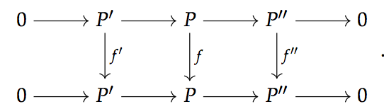
The above definition is not immediately seen to be relevant to our original stated desire to study perturbations, but in the investigations of Dundas and McCarthy of stable $K$-theory, the $K$-theory of endomorphisms naturally comes up. In this paper they prove the following theorem:

Theorem. For $R$ a ring and $M$ a discrete $R$-bimodule)

$$\tilde{K}(R;B_\bullet M) \simeq \text{hofib} \left\{ K(R \oplus M) \rightarrow K(R) \right\} = \tilde{K}(R \oplus M),$$

where $R \oplus M$ is again the the square-zero extension of $R$ by $M$.

We think of $R \oplus M$ as a perturbation of $R$ by $M$, as the elements that we are adding on (those coming from the direct summand $M$) are “so small’’ that they multiply to zero. This result relates the “perturbation’’ approach to understanding $K$-theory to our earlier potential approach of understanding the free objects in the category of augmented $R$-algebras.

That’s great, but we’d like to actually have some idea of what these things are. To get a hint at what we should be looking for, we go back to what was classically studied by Almkvist et al.

$K$-Theory of Endomorphisms: The Classical Story

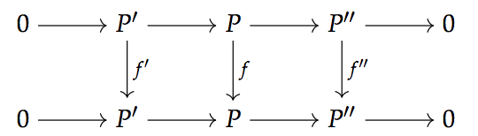
Definition. Let $R$ be a ring and consider the category $End(R)$, whose objects are pairs $(P,f)$ with $P$ a finitely-generated projective $R$-module and $f:P \rightarrow P$ an endomorphism. The morphisms in this category are commutative diagrams of the appropriate type.

Now, we might ask what possible “additive invariants’’ there are on this category, having in mind a few examples. The key (and, as it turns out, universal) one is the following:

Example. [The Characteristic Polynomial] Let $(P,f) \in End(R)$, then the characteristic polynomial of $f$ is given by

$$\lambda_t (f) = \sum_{i \geq 0} Tr(\Lambda^i f)t^i.$$

This can also be obtained in the usual way as a determinant.

The important property of the characteristic polynomial is that if we have a commutative diagram in $End(R)$

with exact rows, then

$$\lambda_t (f) = \lambda_t (f') \cdot \lambda_t (f''),$$

meaning that the characteristic polynomial takes short exact sequences of endomorphisms to products (which are sums in the abelian group where the characteristic polynomials lie).

We now know that a search for additive invariants is a desire to compute $K$-theory, and so we define:

Definition. $K_0 (End(R))$ is defined to be the free abelian group on isomorphism classes of objects in $End(R)$ modulo the subgroup generated by the relations $[(P,f)] = [(P',f')] + [(P'',f'')]$ if there is a commutative diagram

with the rows exact. There is a natural splitting

$$K_0 (End(R)) \simeq K_0 (R) \times \tilde{K}_0 (End(R))$$

coming from thinking of the category of finitely generated projective $R$-modules as living in $End(R)$ as the guys with $0$ endomorphisms.

Of course, $End(R)$ is an exact category, and we could define higher $K$-groups for this as well.

$K_0 (End(R))$ is the repository for additive invariants, in that it has the following universal property:

Proposition. Let $F$ be a map from the commutative monoid of isomorphism classes of objects in $End(R)$ to an abelian group $A$, such that $F$ splits short exact sequences as above. Then $F$ factors through $K_0 (End(R))$, or $K_0(End(R))$ is the initial abelian group for which short exact sequences of endomorphisms split.

What does this look like, though? Well, let’s go back to the characteristc polynomial:

Theorem. The map

$$c: [(P,f)] \mapsto ([P], \lambda_t (f))$$

is an isomorphism

$$K_0 (End(R)) \simeq K_0 (A) \times \tilde{W}(R),$$

where

$$\tilde{W} (R) = \left \{ \dfrac{1 + a_1 t + \dots + a_n t^n}{1+ b_1t + \dots + b_m t^m} ; \; a_i, b_j \in R \right \}$$

is the multiplicative group of fractions with constant term 1.

The moral of this is that the characteristic polynomial encodes all of the additive information about an endomorphism (the trace is a special case of this, of course, being read off by the constant term of the characteristic polynomial). Something interesting is the following:

Proposition. The inclusion $\tilde{W}(R) \rightarrow W(R)$ exhibits $\tilde{K}_0 (R)$ as a dense $\lambda$-subring of $W(R)$, where $W(R)$ are the big Witt vectors of $R$, modelled as power series with constant term $1$.

This means that we might as well think of the big Witt vectors as being limits of characteristic polynomials of endomorphisms, which is the starting point for the line of thought that led to the Lindenstrauss and McCarthy results.

It is also important to mention what some of the uses of this equivalence are:

• Calculations that may be difficult to perform on Witt vectors might be easy if we think of them as coming from characteristic polynomials of endomorphisms;
• Operations that exist on Witt vectors get turned into operations on K-theory, and vice-versa:
• The $n$-th ghost map is given by $gh_n ([P,f] = tr(f^n))$;
• The Frobenius map is given by $F_n ([P,f]) = [P, f^n]$;
• The Verschiebung map is given by $[V_n ([P,f]) = [P^{\oplus n}, v_n f]$, where $v_n f$ is represented by a shift in the first $n-1$ factors and action by $f$ in the last factor. This represents an $n$-th root of $f$, in that $V_n^n$ looks like applying $f$ to all of the blocks of $P^{\oplus n}$.

Lindenstrauss-McCarthy and Topological Witt Vectors

The first thing to do to start generalizing the previous construction is to allow for a “parametrization’’, like we said before.

Definition. Let $R$ be a ring and $M$ an $R$-bimodule. $End(R;M)$ is the category whose objects are pairs $(P,f)$ with $P$ a finitely generated projective $R$-module and $f: P \rightarrow P \otimes_R M$ a map of $R$-modules. As in $End(R)$, morphisms are commutative diagrams.

$End(R;M)$ inherits an exact/Waldhausen structure from considering what’s happening in the “base’’, and so it makes sense to define parametrized $K$-theory as

$$K(R;M) := K(End(R;M)).$$

There is a natural map from $End(R;M)$ to the category of finitely generated projective $R$-modules that forgets the endomorphism, and so we can reduce and consider

$$\tilde{K}(R;M) := hofib(K(R;M) \rightarrow K(R)).$$

We can also consider $M$ to be simplicial by geometrically realizing, and this assembles to a functor

$$\tilde{K}(R;-): \left\{\text{simplicial } R\text{-bimodules} \right \}\; \rightarrow \text{Spectra},$$

which is a good setting to do Goodwillie calculus.

The remarkable result of Lindenstrauss-McCarthy is the following:

Theorem. The functors $\tilde{K} (R; -), W(R;-)$ from simplicial $R$-bimodules to spectra have the same Taylor tower, where $W(R;-)$ is a “topological Witt vectors’’ construction.

Now, this is only remarkable if I tell you what this $W(R;-)$ functor is, so let’s do that. Lindenstrauss and McCarthy describe this using the (notationally cumbersome) language of FSPs instead of spectra or spectral categories, which makes everything a bit hard to read. The idea is a bit simpler, however.

Construction. Let $R$ be a ring, $M$ a bimodule. We define a bunch of spectra $U^n (R;M)$ with $C_n$ action by letting $U^n (R;M)$ be the derived cyclic tensor product (over $R$) of $n$ copies of $M$.

There is an evident $C_n$ action on $U^n (R;M)$ given by permuting the factors, and moreover when $n \mid N$, we have natural restriction maps between the fixed points

$$res : U^N (R;M)^{C_N} \rightarrow U^n (R;M)^{C_n}.$$

We then define

$$W(R;M) := holim_{res} U^n (R;M)^{C_n}.$$

Example. $U^1 (R;M) \simeq THH(R;M)$ as normally defined, and if $R = M$ then we have that $W(R;M) \simeq TR(R;M)$.

This functor $W(R;M)$ is meant to be an attempt to define $TR$ in the absence of the cyclic symmetry that is present when $M = R$. The remarkable thing is that this actually works! The nomenclature is justified by the following $p$-typical statement:

Theorem. (Hesselholt-Madsen) $\pi_0 (TR(R;p)) \simeq W_{(p)}(R),$

where the latter is a suitable version of $W(R;M)$ that takes a homotopy limit over only $U^{p^n}(R;M)^{C_{p^n}}$.

The virtue of this setup is that we have explicit understanding of what the layers of the Taylor tower of $W(R;-)$ look like, as well as various splitting theorems, e.g. we have the following ``fundamental cofibration sequence’’:

Theorem. There is a homotopy fiber sequence

$$U^n (R; M)_{hC_n} \rightarrow W^{n}(R; M) \rightarrow W^{(n-1)}(R; M),$$

where $W^{n}(R;M)$ are the functors obtained by truncating the homotopy limit defining $W(R;M)$.

Moreover, we have that $W^{n}(R;M)$ is the $n$th polynomial approximation of $W (R;M)$, so this is the fiber sequence that computes the layers of the Taylor tower.

Generalizations

The problem with the Lindenstrauss-McCarthy story is that it is only proven for discrete rings, but all of the constructions floating around can just as well be made when $R$ is a connective ring spectrum and $M$ is a (simplicial) $R$-bimodule.

One of the great tricks that one can do is to use the resolution of connective ring spectra by simplicial rings. That is, given a connective ring spectrum $R$, there is a $id$-Cartesian cube with initial vertex $R$, and such that all other vertices are canonically stably equivalent to the Eilenberg-MacLane spectrum of a simplicial ring.

The following fact lets us promote results about simplicial rings to those about connective ring spectra:

Theorem. If $\chi$ is an $(id)$-Cartesian $k$-cube of connective ring spectra, then the cube $K(\chi)$ is $(k+1)$-Cartesian.</span>

Idea for proving generalization: Show that the functors $W(-;-), \tilde{K}(-;-)$ have a similar property, so that the equivalence given by Lindenstrauss and McCarthy can be promoted to one for connective ring spectra.

This works just fine, and we arrive at:

Theorem. (P.) The Lindenstrauss-McCarthy result hnews for connective ring spectra.

Unfortunately, this is mostly just a one-off trick, and we are still looking for a good conceptual understanding of what the Lindenstrauss-McCarthy equivalence really means. It largely goes back to the Dundas-McCarthy theorem mentioned earlier, which can also be proven for connective ring spectra, but fails to admit a generalizable proof. The issue that arises there is that their proof relies heavily on the linear models of $K$-theory when working over discrete rings, and these simply faily to work when we move to other contexts (their proof involves the addition of maps, a simplicial model of $K$-theory, etc.).

If we had a good way of dealing with the coherence issues in defining the Dundas-McCarthy maps, then we might be able to generalize the proof and understand what’s going on, but that’s something that has yet to be done.

A Serif blog | View archive of 36 posts